Data Analysis of Indoor thermal environment

1. Introduction

This project was developed for a research topic at Tokyo Tech’s Yasuda Laboratory. It involves visualizing indoor thermal environment data of buildings using Seaborn, sklearn, and pandas, and conducting Random Forest Classification on various factors to identify the main factors affecting the indoor thermal environment.

Google Colab Link

Data Source: Official Github

2. Environment

Python (Pandas, Seaborn, Sklearn)
Jupyter Notebook

3. Analysis Process

3.1 Reading Data

The first thing we need to do is create the the feature data set and the target variable.
Let’s use the following columns as input features for the classification model. These features will be used by the model to try to predict `ThermalSensation_rounded`.
Several of the features are related to the building context (i.e.: `Country`, `City`), the environmental conditions (i.e.: `Air Temperature (C)`, `Relative humidity (%)`) and personal factors (i.e.: `Sex`, `Clo`, etc.)
The target variable is the column that we want to predict – in this case, thermal sensation. We will use the “rounded” version to minimize the number of categories

				
					ieq_data = pd.read_csv("ashrae_thermal_comfort_database_2.csv", index_col='Unnamed: 0')
ieq_data.info()
ieq_data["ThermalSensation_rounded"].value_counts()
feature_columns = [
 'Year',
 'Season',
 'Climate',
 'City',
 'Country',
 'Building type',
 'Cooling startegy_building level',
 'Sex',
 'Clo',
 'Met',
 'Air temperature (C)',
 'Relative humidity (%)',
 'Air velocity (m/s)']
 features = ieq_data[feature_columns]
 features.info()
 target = ieq_data['ThermalSensation_rounded']

3.2 Create dummy variables for the categories

We need to convert the categorical variables to dummy variables(similar to one-hot coding but simpler) in order as that is the input the model expects
Now we will create a function that will divide the data set into a random train/test combination.
Let’s call the Random Forest model from sklearn that was loaded before and specify various input features (or parameters) that influence the way the model is constructed.

				
					features_withdummies = pd.get_dummies(features)
features_withdummies.head()
features_train, features_test, target_train, target_test = train_test_split(features_withdummies, target, test_size=0.3, random_state=2)
model_rf = RandomForestClassifier(oob_score = True, max_features = 'auto', n_estimators = 100, min_samples_leaf = 2, random_state = 0)
model_rf.fit(features_train, target_train)

The model is accurate about half the time in predicting if someone is comfortable. It is low now, but let’s find where the baseline is. A baseline which is the accuracy in just random guessing

				
					#Dummy Classifier model to get a baseline
baseline_rf = DummyClassifier(strategy='stratified',random_state=0)
baseline_rf.fit(features_train, target_train)

baseline_model_accuracy = baseline_rf.score(features_test, target_test)
print("base accuracy: "+str(baseline_model_accuracy))

Year	Clo	Met	Air temperature (C)	Relative humidity (%)	Air velocity (m/s)	Season_Winter
2012	0.75	1	25.2	64	0.1	1
2012	0.64	1	25.2	64	0.1	1
2012	0.64	1	25.2	64	0.1	1
2012	0.75	1	25.2	64	0.1	1
2012	0.72	1	25.2	64	0.1	1

3.2 Classification Report

Classification is often evaluated by more than just accuracy — there are several other metrics that are calculated to understand the success to classification. We can report that outlines the precision, recall, f1-score, and support metrics for each of the classes being predicted.

				
					y_pred = model_rf.predict(features_test)
y_true = np.array(target_test)
categories = np.array(target.sort_values().unique())
print(classification_report(y_true, y_pred))

3.3 Feature Importance

With Random Forest models, there is the built-in capability to calculate the Feature Importance to know which element really matter for built envirnoment.
According to the feature importance analysis, it seems that the conventional environmental metrics(Air temperature, Relative humidity, Air velocity) are the best predictors of comfort followed by the personal factors

				
					importances = model_rf.feature_importances_
std = np.std([tree.feature_importances_ for tree in model_rf.estimators_], axis=0)
indices = np.argsort(importances)[::-1]
# Print the feature ranking
print("Feature ranking:")
for f in range(10):
    print(f + 1, features_withdummies.columns[indices[f]], importances[indices[f]])

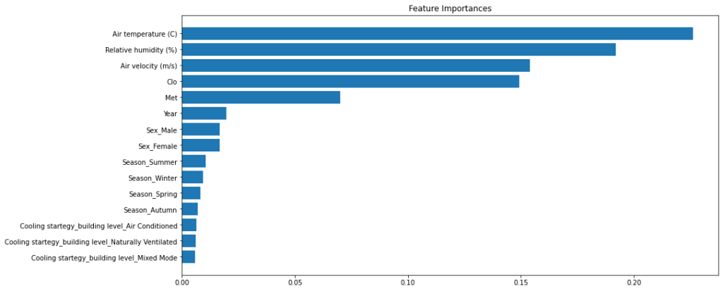
Rank	Feature	Importance
1	Air temperature (C)	0.2261
2	Relative humidity (%)	0.1920
3	Air velocity (m/s)	0.1540
4	Clo	0.1494
5	Met	0.0700
6	Year	0.0195
7	Sex_Male	0.0167
8	Sex_Female	0.0166
9	Season_Summer	0.0106
10	Season_Winter	0.0094

3.3 Plot Feature Importance

We can also plot the feature importance in a line chart of the top features to get a better visual sense

				
					# Plot the feature importances of the forest
plt.figure(figsize=(15,6))
plt.title("Feature Importances")
plt.barh(range(15), importances[indices][:15], align="center")
plt.yticks(range(15), features_withdummies.columns[indices][:15])#
plt.gca().invert_yaxis()
plt.tight_layout(pad=0.4)
plt.show()